Activation functions

Well, basically what we have done so far is represent our different input features and their weights in a lower dimension, as a scalar representation. We can use this reduced representation and pass it through a simple non-linear function that tells us whether our representation is above or below a certain threshold value. Similar to the weights we initialized before, this threshold value can be thought of as a learnable parameter of our perceptron model.

In other words, we want our perceptron to figure out the ideal combinations of weights and a threshold, allowing it to reliably match our inputs to the correct output class. Hence, we compare our reduced feature representation with a threshold value, and then activate our perceptron unit if we are above this threshold value, or do nothing otherwise. This very function that compares our reduced feature value against a threshold, is known as an activation function:

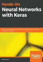
These non-linear functions come in different forms, and will be explored in further detail in subsequent chapters. For now, we present two different activation functions; the heavy set step and the logistic sigmoid activation functions. The perceptron unit that we previously showed you was originally implemented with such a heavy step function, leading to binary outputs of 1 (active) or 0 (inactive). Using the step function in our perceptron unit, we observe that a value above the curve will lead to activation (1), whereas a value below or on the curve will not lead to the activation unit firing (0). This process may be summarized in an algebraic manner as well.

The following screenshot shows the heavy step function:

The output threshold formula is as follows:

In essence, a step function is not really a non-linear function, as it can be rewritten as two finite linear combinations. Hence, this piece-wise constant function is not very flexible in modeling real-world data, which is often more probabilistic than binary. The logistic sigmoid, on the other hand, is indeed a non-linear function, and may model data with more flexibility. This function is known for squishing its input to an output value between 0 and 1, which makes it a popular function for representing probabilities, and is a commonly employed activation function for neurons in modern neural networks:

Each type of activation function comes with its own set of advantages and disadvantages that we will also delve into in later chapters. For now, you can intuitively think about the choice of different activation functions as a consideration based on your specific type of data. In other words, we ideally try to experiment and pick a function that best captures the underlining trends that may be present in your data.

Hence, we will employ such activation functions to threshold the incoming inputs of a neuron. Inputs are consequentially transformed and gauged against this activation threshold, in turn causing a neuron to fire, or abstain therefrom. In the following illustration, we can visualize the decision boundary produced by an activation function.