How it works...

The following is the explanation of the code and how it works:

• fig, axs = plt.subplots(1,3, figsize=(9,6)) defines the figure layout with three plots in a row, with a figure size of (9, 6). 
• fig.subplots_adjust(left=0.0, bottom=0.05, right=0.9, top=0.95, wspace=0.6) defines the bounding box for the figure leaving space on all four directions as defined on the left, bottom, right, and top of the figure. wspace defines the amount of space to be left in between the plots in a row so that there is no overlap between their labels or plots. hspace is another parameter that controls the space between the plots in a column. We have not used it in this example, as we are plotting all the graphs in one row only.
• plot_graph() is a user-defined function to plot the graph with the given arguments, axes, colormap, and color bar axes.
• axs.scatter() plots a scatter plot using the given arguments. caxs = plt.axes(cbaxs) defines the color bar at the given axes, co-ordinates. fig.colorbar() plots the color bar with three ticks for each of the clusters with a defined color, and labels the color bar with cluster #.
• We plot the first graph on axes[0], the first three colors of the pre-defined colormap coolwarm, and colorbar axes cbaxs =[0.24, 0.05, 0.03, 0.85]. These are the fractions of the figure from left and bottom, and the width and the height of the bar. We will learn more about co-ordinate systems in Chapter 6, Plotting with Advanced Features.
• We plot the second graph on axes[1], with custom colors colors = [(1, 0, 0), (0, 1, 0), (0, 0, 1)], which are pure red, green, and blue.
• cmap_name = 'custom_RGB_cmap' defines the name for the first user-defined colormap. This will be useful if we have to register it to be included in the standard colormaps library.
• cm = LinearSegmentedColormap.from_list(cmap_name, colors2, N=3) defines the colormap with the list of three colors defined previously. 
• For the second graph, we place the color bar at these co-ordinates: cbaxs = [0.58, 0.05, 0.03, 0.85].
• Similarly, we plot the third graph with colors = [(1, 0.5, 0), (0.25, 0.5, 0.25), (0.8, 0.8, 0.25)] and place them at co-ordinates cbax = [0.95, 0.05, 0.03, 0.85]. The colors in each of the red, green, and blue channels are again mixed with a combination of red, green, and blue of different values to create new custom colors. 

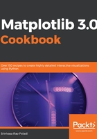
You should see the following plots: